Quick start: Forecasting with synthetic data

In this notebook, we train Treeffuser on synthethic data and then visualize both the original and model-generated samples to explore how well Treeffuser captures the underlying distribution of the data.

Getting started

We first install treeffuser and import the relevant libraries.

%%capture
!pip install treeffuser

import matplotlib.pyplot as plt
import numpy as np

from treeffuser import Treeffuser

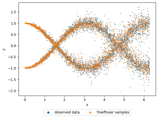
We simulate a non-linear, bimodal response of \(y\) given \(x\), where the two modes follow two different response functions: one is a sine function and the other is a cosine function over \(x\).

seed = 0  # fixing the random seed for reproducibility
n = 5000  # number of data points

rng = np.random.default_rng(seed=seed)
x = rng.uniform(0, 2 * np.pi, size=n)  # x values in the range [0, 2π)
z = rng.integers(0, 2, size=n)  # response function assignments

y = z * np.sin(x - np.pi / 2) + (1 - z) * np.cos(x)

We also introduce heteroscedastic, fat-tailed noise from a Laplace distribution, meaning the variability of \(y\) increases with \(x\) and may result in large outliers.

y += rng.laplace(scale=x / 30, size=n)

Fitting Treffuser and producing samples

Fitting Treeffuser and generating samples is very simple, as Treeffuser adheres to the sklearn.base.BaseEstimator class. Fitting amounts to initializing the model and calling the fit method, just like any scikit-learn estimator. Samples are then generated using the sample method.

model = Treeffuser(sde_initialize_from_data=True, seed=seed)
model.fit(x, y)

y_samples = model.sample(x, n_samples=1, seed=seed, verbose=True)

100%|██████████| 1/1 [00:01<00:00,  1.02s/it]

Plotting the samples

We create a scatter plot to visualize both the original data and the samples produced by Treeffuser. The samples closely reflect the underlying response distributions that generated the data.

plt.scatter(x, y, s=1, label="observed data")
plt.scatter(x, y_samples[0, :], s=1, alpha=0.7, label="Treeffuser samples")

plt.xlabel("$x$")
plt.ylabel("$y$")

legend = plt.legend(loc="upper center", scatterpoints=1, bbox_to_anchor=(0.5, -0.125), ncol=2)
for legend_handle in legend.legend_handles:
    legend_handle.set_sizes([32])  # change marker size for legend

plt.tight_layout()

The samples generated by Treeffuser can be used to compute any downstream estimates of interest.

x = np.array(np.pi).reshape((1, 1))
y_samples = model.sample(x, n_samples=100, verbose=True)  # y_samples.shape[0] is 100

# Estimate downstream quantities of interest
y_mean = y_samples.mean(axis=0)  # conditional mean for each x
y_std = y_samples.std(axis=0)  # conditional std for each x

print(f"Mean of the samples: {y_mean}")
print(f"Standard deviation of the samples: {y_std} ")

100%|██████████| 100/100 [00:00<00:00, 435.02it/s]

Mean of the samples: [-0.05467086]
Standard deviation of the samples: [0.99499814]

For convenience, we also provide a class Samples that can estimate standard quantities.

from treeffuser.samples import Samples

y_samples = Samples(y_samples)
y_mean = y_samples.sample_mean()  # same as before
y_std = y_samples.sample_std()  # same as before
y_quantiles = y_samples.sample_quantile(q=[0.05, 0.95])  # conditional quantiles for each x

print(f"Mean of the samples: {y_mean}")
print(f"Standard deviation of the samples: {y_std} ")
print(f"5th and 95th quantiles of the samples: {y_quantiles.reshape(-1)}")

Mean of the samples: [-0.05467086]
Standard deviation of the samples: [0.99499814]
5th and 95th quantiles of the samples: [-1.25918297  1.06402459]